Decay Functions
Introduction
Conveyal Analysis can apply decay functions rather than hard cutoffs in both regional and single-point analyses. Rather than being the sum of all opportunities that can be reached in less than a specified number of minutes, an accessibility indicator can be more generally defined as the sum of all opportunities in the region, with each opportunity weighted (multiplied) by the value of a "decay function". This function always returns values between zero and one, and is a monotonically decreasing function of travel time. Put differently, the longer it takes to reach each opportunity the less it counts, eventually tapering down to zero. Simple cumulative opportunities accessibility is then a special case of this general definition where the weighting function has value 1 for all travel times less than the threshold, and value 0 for all travel times at or above the threshold.
If you think of accessibility as the number of opportunities falling inside an isochrone, then the effect of gravity-style decay functions is to blur the boundary of that isochrone. The influence of large concentrations of opportunities on accessibility values is diffused. The opportunities fade out with increasing travel time from the origin, rather than simply "dropping out" of the isochrone or "falling off the edge".
In choosing a decay function, there is a trade-off between ease of explanation and fidelity to traveler behavior. Simple cumulative opportunities accessibility indicators are easy to explain and interpret. A definition like "number of jobs reachable in less than 30 minutes" poses little risk of confusing an audience or sidetracking a meeting into a mathematical discussion. However, these indicators are very sensitive to the exact cutoff chosen. A large office park situated 31 minutes away might contribute nothing to the accessibility value of a particular origin point. But the reachable jobs count could increase sharply at a neighboring origin point, from which the same office park happens to be 29 minutes away. This creates discontinuities in the accessibility surface and differs from how most people perceive travel.
Consider another example with a 30-minute hard cutoff, where a scenario with a new link reduces travel time from a given origin to all destinations by 5 minutes (relative to a baseline scenario). From this origin, destinations that were previously 25 minutes away would be reachable in both cases, so they would not affect the chosen access metric; similarly, destinations that were previously 45 minutes away would be unreachable in both cases, so they would not affect the chosen access metric. The only benefits with a step function and a 30 minute cutoff would arise from a narrow band of opportunities that were previously 31-35 minutes away (and are now reachable in 26-30 minutes). The logistic decay function uses the idea of a threshold, but with a wider band that allows more destinations to affect the resulting indicator.
Before the introduction of decay functions, Conveyal Analysis dealt with this sensitivity by emphasizing interactive changes to the cutoff: in single point analyses you can readily shift the cutoff by a minute or two to ensure that an accessibility figure you're observing is not at an unstable location or time. Decay functions provide an alternate strategy for confronting this issue, as well as the important fact that some travelers will tolerate much higher travel times than others: decay functions may be interpreted as applying different step cutoffs for different proportions of the population.
All decay functions are evaluated at one-second resolution, so the weights applied to the opportunities decrease very smoothly. Although Analysis reports travel times in minutes, they are internally measured in seconds.
Configuration and Use
The default function applied in any new request is the step function, equivalent to the hard cutoff. It is possible to select a different decay function in the request settings of the single-point analysis tab and set that function's parameters (controlling the shape and steepness of the downward slope). These choices will be passed on to any regional analysis that you run. You should see the effects of the chosen decay function reflected in the cumulative accessibility plot, generally creating a smoother curve than a step function does.
As with most other options, decay functions can also be specified in the advanced request JSON editor. Examples of JSON are given below along with descriptions of each available decay function.
Available Functions
Logistic CDF
This is the logistic function, i.e. the cumulative distribution function of the logistic distribution, expressed such that its parameters are the median (inflection point) and standard deviation. This function applies a sigmoid rolloff that has a convenient relationship to discrete choice theory. Its parameters can be set to reflect a whole population's tolerance for making trips with different travel times. The function's value represents the probability that a randomly chosen member of the population would accept making a trip, given its duration. Opportunities are then weighted by how likely it is a person would consider them "reachable".
The median parameter is controlled by Conveyal's cutoff setting, leaving only the standard deviation to configure. In the advanced JSON editor this appears as:
"decayFunction": {
  "type": "logistic",
  "standardDeviationMinutes": 5
}
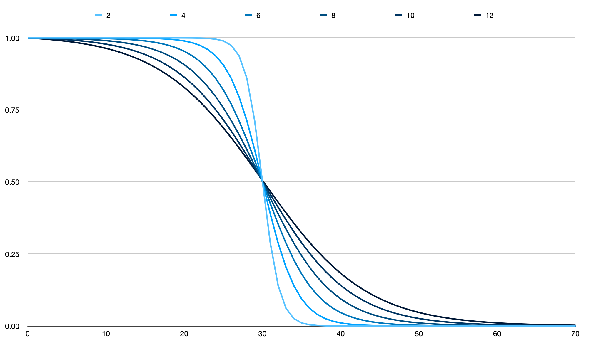
This is the family of curves produced at different cutoffs when the standardDeviationMinutes is set to 10:
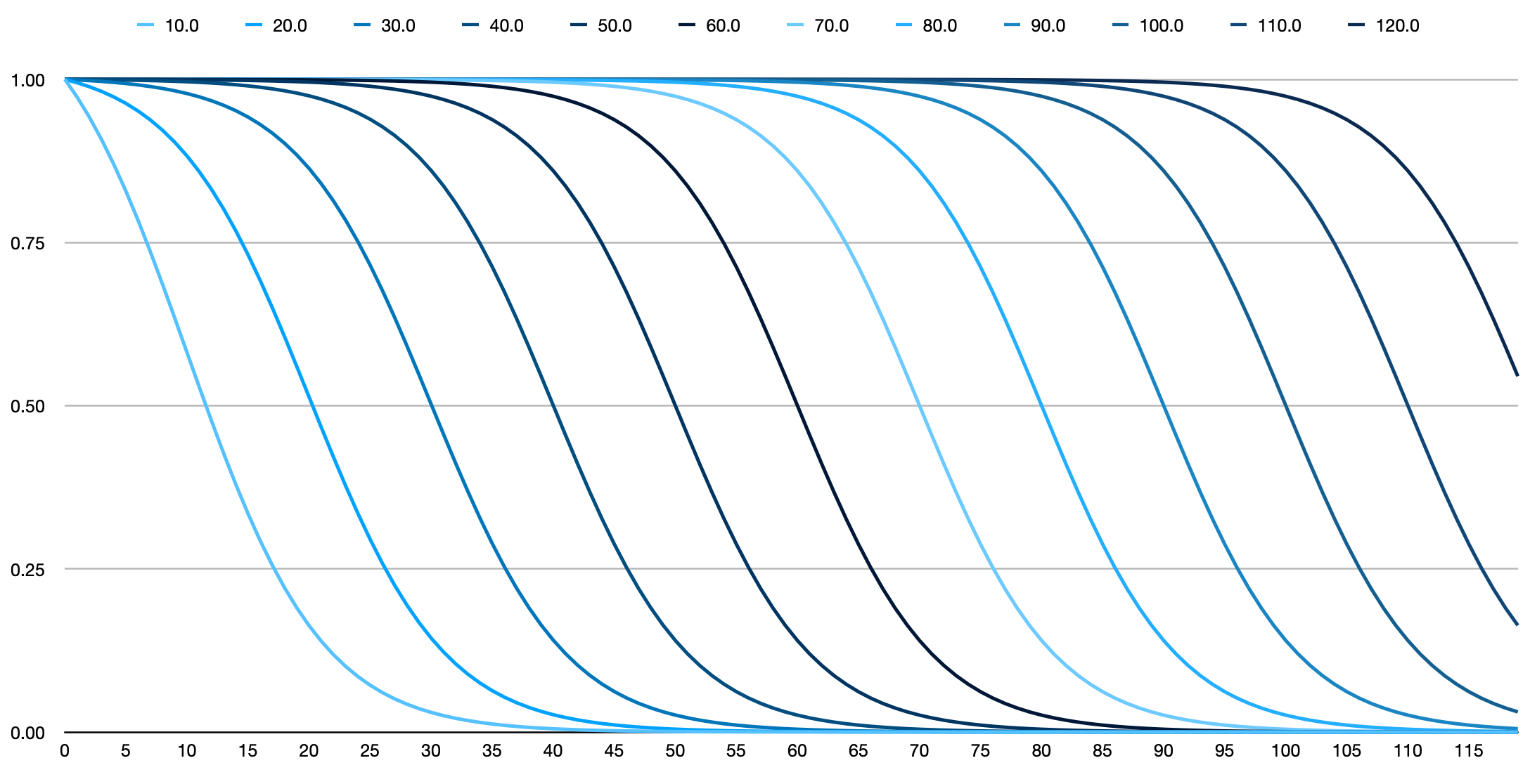
The following plot shows how the form of the function varies as the standard deviation is changed. The median here is 30 minutes. The function remains generally similar in form at other cutoffs, though as you can see from the previous plot it changes a bit with cutoffs close to zero.
Fixed Exponential Decay
Please note that the exponential decay option visible in the Conveyal web app refers to the half-life exponential decay function described below. The fixed-decay form described in this section can only be specified manually via JSON.
This function is of the form e-λt where λ is a single fixed decay constant in the range (0, 1). The constant is constrained to be positive to ensure weights decrease (rather than grow) with increasing travel time. The decay constant should be scaled for travel times in seconds. If your decay constant is for travel times in minutes, you will need to divide it by 60. This function can be specified in the advanced JSON view as follows:
"decayFunction": {
  "type": "fixed-exponential",
  "decayConstant": 0.001
}
Unlike the other functions, this function will ignore the cutoff setting in Conveyal Analysis. This allows setting precise decay constants derived from your own models or research that do not correspond to an integer half-life in minutes. The cutoff will not affect the rate of decay or transpose the function in any way. For this reason, only one cutoff should be specified when launching a regional analysis, and that cutoff is arbitrary. Any additional cutoffs will perform extra computation but yield exactly the same results. Different percentiles will continue to affect the results - selecting different percentiles will yield different travel times to each destination, with increasing travel times giving lower weights to opportunities at those locations.
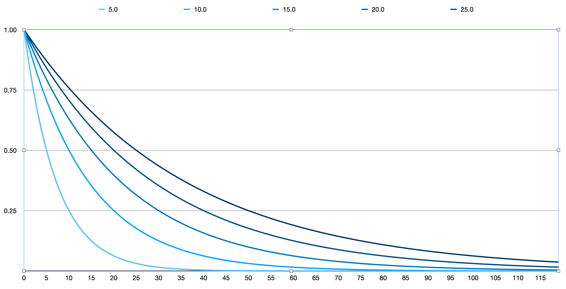
Exponential Decay
This is similar to the fixed-exponential option above, but in this case the decay parameter is inferred from Conveyal's cutoff setting, which is treated as the half-life. It has no other parameters and is specified like this:
"decayFunction": {
  "type": "exponential"
}
This plot shows how the shape of the exponential decay changes in response to different half-lives:
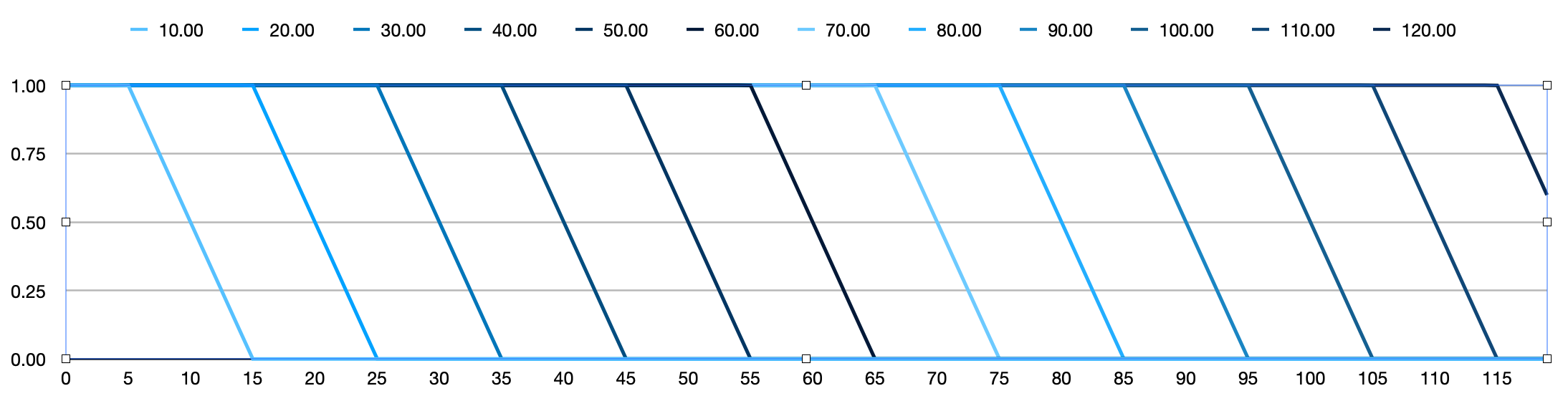
Linear
This is a simple, vaguely sigmoid option, which may be useful when you have a sense of a maximum travel time that would be tolerated by any traveler, and a minimum time below which all travel is perceived to be equally easy. It is a bit more computationally efficient than the logistic CDF, as it truly reaches zero and the routing engine can skip searching for paths beyond the zero point. It is configured as follows in JSON:
"decayFunction": {
  "type": "linear",
  "widthMinutes": 10
}
The transition region is transposable and symmetric around the cutoff, taking widthMinutes to taper down from one to zero. The above configuration with widthMinutes equal to 10 gives the following family of linear decay functions: