Single point analysis
The main analysis page is for generating isochrones (travel time contours) from selected origins. To enter analysis mode, click the icon on the sidebar.
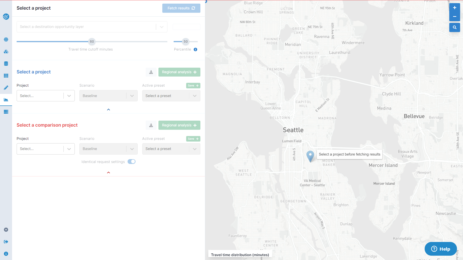
To start an analysis, you'll need to select a project and scenario. Once these are selected you can fetch results for the origin marker shown on the map either by moving the marker to a new location or clicking Fetch results
This will initialize a compute cluster which may take a minute to start up. If this is your first time performing an analysis with a given network bundle it may take some time to build the network, however this only needs to be done once for each bundle. For more information, see the FAQ page.
Once the compute cluster is initialized you should see an isochrone displayed in blue around your point on the map. If you have selected an destination opportunity layer, you will also see a chart of accessibility at selected time and percentile thresholds. You may also select a comparison project and scenario, which will be shown in red. Many other configuration parameters are described in the Options and Configuration.
Isochrone map
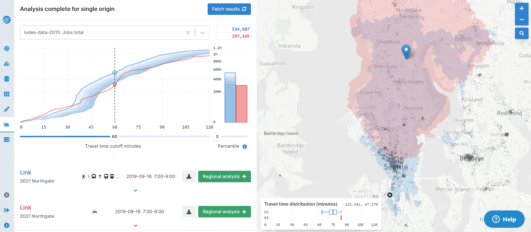
After the server returns results the map will show a blue isochrone for your primary scenario. This represents the area reachable from the origin marker within the selected travel time cutoff, to a given degree of certainty. If a comparison scenario is selected, its isochrone will be shown in red. The overlap of the main and comparison isochrones should be visible as a combination of the two colors.
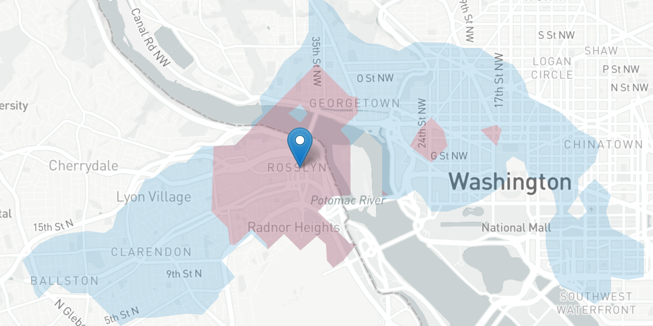
The travel time cutoff slider controls the travel time threshold between a range of one minute and two hours. The slider for travel time percentile controls the portion of departures within the time window that have to meet the travel time threshold. Reducing the travel time should smoothly decrease the size of the isochrone. The default values are 60 minutes, at the 50th percentile. This would mean that the default isochrone boundary is drawn where the median trip in the selected departure window would take exactly one hour.
For results that include uncertainty and variability due to transit schedules, changing the travel time percentile slider will change the isochrones, destination travel time legend, and accessibility charts accordingly. See the methodology page for more details.
For single point analysis, travel time percentile is limited to five default values (5, 25, 50, 75, 95). Arbitrary percentile values can be set for a regional analysis.
To change the origin of the analysis, drag the marker to a new location.
The display of modifications on the map is controlled in editing mode (See: Toggling display of modifications). To change what modifications are shown, you must set the visibility there and then navigate back to the analysis page.
Travel time and itinerary details
Conveyal provides unique ways to check the variability of transit trips and detailed itineraries.
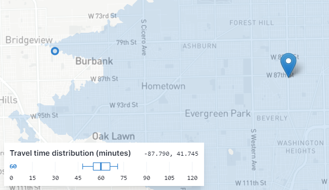
To visualize the distribution of total travel times to a specific destination, click the icon in the destination legend (lower left). A small circular destination marker will then follow your cursor across the map, and the legend will update with a plot of travel time at the five default percentile values listed above. For example, in the image below the travel time varies between about 30 and 50 minutes depending on when one departs (and the random schedules simulated if frequency-based routes are present). Click on the map to pin the destination marker to a specific location, which can be useful for comparing travel times from different origins or for different requests. Click on a pinned destination marker to make it follow your cursor again.
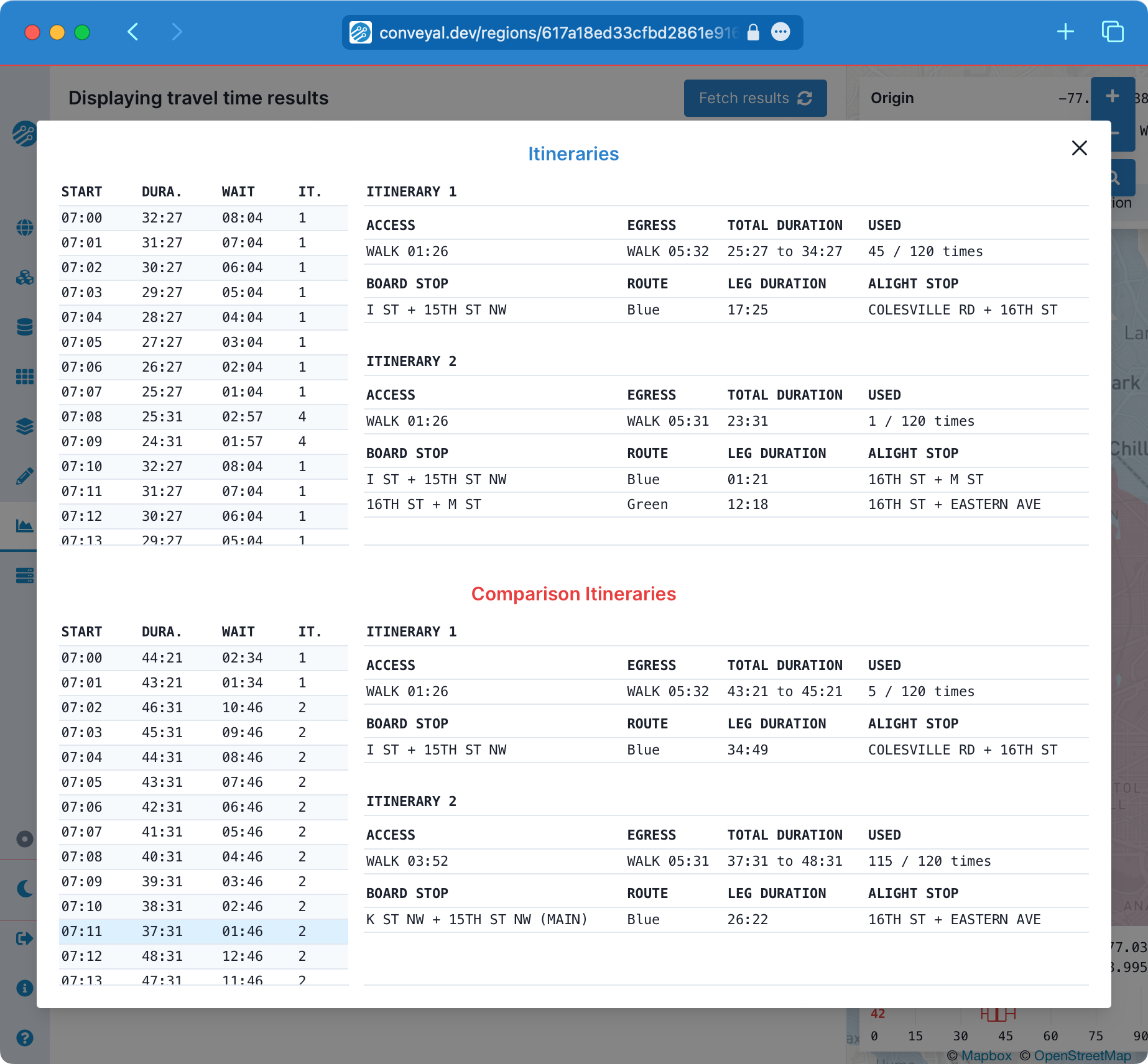
To view itinerary details, pin the destination marker as described above and click "Fetch Results." Once results are returned, click "View routes to destination," which appears in the origin legend (upper left).
In the itinerary viewer, the left table shows a minute-by-minute summary of optimal itineraries from your selected origin to destination. Details for each itinerary are on the right, including access/egress time/modes, a range of total door-to-door durations (reflecting different waiting times encountered), how many iterations the itinerary was used for, and information about each transit leg of the journey (boarding/alighting stops, route, and in-vehicle time). This feature is not available for routing engine versions prior to v6.8.
Analysis panel
The left panel has controls for the analysis and displays the access to opportunities afforded by the selected scenarios. If network modifications are included in a scenario, certain details (such as the number of transit trips or street network edges affected) may be listed at the top of this panel.
Available spatial datasets are listed in the drop-down menu for selection as a destination layer. For example, you might be interested in how a given scenario provides access to jobs, schools, or some other opportunity of interest.
The grid cell zoom level allows you to select the spatial resolution used for analysis. The resolution applies to the destination grid in single-point analysis, and only spatial datasets with the same zoom level can be selected as destination opportunities. In regional analyses, the resolution applies to the origin grid, and destination grids can be a different zoom level. Higher zoom levels imply substantially more computation and may require you to reduce the boundaries of your analysis.
Below the travel time slider, sub-panels allow selection of projects, scenarios, and different analysis settings. A baseline scenario with no modifications (i.e. the unmodified network bundle you uploaded) is automatically available for every project.
The options available in these sub-panels are described more fully in Options and Configuration.
Chart of accessibility results
If a spatial dataset is selected as a destination opportunity layer, the map will show a dot-density layer of these opportunities, and the analysis panel will show the number of opportunities accessible from the origin selected on the map.
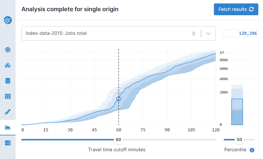
Below the spatial dataset selector and accessibility result for the selected travel time cutoff, a stacked percentile plot shows the cumulative number of opportunities reachable at different travel time cutoffs. When transit schedules introduce variability, the graph will not be a single line because travel times (and consequently, accessibility) depend on when exactly a user of the transport system leaves their origin. In these cases, the graph shows the number of opportunities given the five default percentile travel time values. The bottom of the shaded area is the number of opportunities which are almost always reachable (at 95th percentile travel times), while the top is the number of opportunities that are reachable only in the best cases (at 5th percentile travel times, e.g. when someone leaves their house at the perfect time and has no waiting time, minimizing the overall travel time). The darkened line corresponds to the selected travel time percentile.
When the cumulative plot is steep, areas with especially high opportunity densities (e.g. typical downtown areas for jobs) are reachable. Note that the Y axis is a square-root scale, so that the cumulative plot would be a straight line if both the opportunities and travel speeds radiating in all directions from an origin were uniform.
The currently-selected travel time cutoff is indicated by the vertical dashed line on the plot.
The stacked bar chart to the right of the cumulative plot shows the same information, but only for the currently selected travel time cutoff. The line around the stacked bars corresponds to the selected travel time percentile.
When a comparison scenario is selected, it will be shown in red on the cumulative plot and the stacked bar chart.
Downloading
Click the download icon () next to your main or comparison scenarios to download the results as a GeoJSON, GeoTIFF, or CSV.
- GeoJSON saves the a multipolygon geometry of the isochrone currently shown on the map. The downloaded file can be converted to other formats using a tool like mapshaper. Note that these vector isochrones are interpolations of the underlying analysis grid.
- GeoTIFF saves the underlying travel time surface, a raster of travel times (in minutes) from the selected origin to the rest of the region. This raster has five bands corresponding to time percentiles of 5, 25, 50, 75, and 95. For geoprocessing, we often suggest using band 3 (the median travel time) of this raw output. Cells beyond the 120 minute cutoff are assigned a value of zero.
- CSV saves a comma-separated table listing the total number of opportunities accessible at all combinations of time and percentile. It has one column for each minute between 1 to 120 and a row for each default percentile value (5, 25, 50, 75, 95).